IVOA Obscore Extension for Radio data#

Status:: ObsCoreExtensionForRadioData 1.0 PEN 2025-09-15

Acknowledgments#

The authors would like to thank all the participants in DM-WG and Radioastronomy-IG discussions for their ideas, critical reviews, and contributions to this document. We acknowledge also the support of ESCAPE (European Science Cluster of Astronomy and Particle Physics ESFRI Research Infrastructures) funded by the EU Horizon 2020 research and innovation program (Grant Agreement no 824064).

1 Introduction#

ObsCore specification ObsCore defines both a minimal datamodel to describe datasets and a table consistent with the model which can be served by TAP services. It has been successful to define a lot of data discovery services in astronomy.

The emergence of the Radioastronomy Interest Group in the IVOA in April 2020 confirmed the strong interest of the radio astronomy community to distribute their data in the VO. Many teams now distribute their data using VO standards [1]. While reduced radio data products, such as images or spectral cubes, are mostly covered by the ObsCore model, the lower level observational data (interferometric visibilities, single dish data in SDFITS, filterbank or whatever other specific formats) require additional description parameters. For interferometry, this need was already exposed in 2010 by Anita Richards in a IVOA Note “Radio interferometry data in the VO” [2] which captures precisely the requirements in the radio community.

Various discovery use cases have been collected in the radio community and gathered in the ObsCoreExtensionForRadioData:ADQLusecases appendix. The current specification suggests addition of new features in the ObsCore metadata profile to fill the gap. With the expansion of large radio astronomy projects such as LOFAR, NenuFAR, the future SKA, ngVLA, etc… and the emergence of interesting research topics matching data in all electromagnetic regimes, the Virtual Observatory framework can facilitate a wider access to radio data for experts and non-specialists radio astronomers in order to support collaborations in multi-wavelength, multi-messenger astronomy.

image

This Radio ObsCore extension in the IVOA, relies on ObsCore itself and expands it to allow data providers to describe their radio data further the ObsTAP framework. Its goal is to clarify how ObsCore metadata can be used in the radio context and to add new specific features to the existing ObsCore metadata.

2 Radio data specifities from the Data Discovery point of view#

On the lower end of the radio spectrum, radio astronomers generally make use of frequencies for designating the spectral ranges of their observation. The standard ObsCore attributes em_min, em_max are expressed in wavelength and are not really convenient. That’s why we should also provide a mechanism for translation into frequencies .But this should not be done by duplicating the same information in two different attributes.

Receivers with a (ultra)wide bandwidth, up to tens of GHz, are nowadays commonly used for both interferometric and Single Dish (herefater SD) radio observations. Given that the spatial field of view and resolution linearly depend on wavelength, these quantities may significantly vary across the observed bandwidth in a radio observation. Generally only a representative value (for instance the receiver nominal frequency) for these two parameters can be given. It is noticeable that this is the case for any measuring system allowing a large interval of \(\lambda/D\) (where \(\lambda\) and \(D\) are the wavelength and the measuring system aperture scale).

Similarly, the resolution power quantity, commonly provided to describe optical spectroscopic data, is generally not used in the radio domain. Instead one could introduce a new ObsCore element for the absolute spectral resolution, in frequency unit, for which a representative value for each observation can be given.

Modern radio instrumentation offers the possibility of several spectral windows within the same observation with significant separation or different resolutions. Such observations may be represented at the highest granularity as a set of combined data sets represented by several entries in an ObsCore table. However it’s up to data provider to decide which level of granularity is best adapted in order to optimize data discoverability and ease data access, depending on the scientific content of the observation.

2.1 Single dish data#

Single Dish (SD) observations can be done with different types of receiving systems. Typical frontends are mono-feed, multi-feed and phased array feed (PAF), the last two suitable to efficiently span wider parts of the sky. Data can be acquired by various backend systems providing either the total intensity (integrated over the whole available bandwidth) or the spectroscopic/spectropolarimetric intensity (acquired in each spectral channel/sample). Data are saved as raw counts resulting from the digitization of the voltage signal measured by the receiving system. Commonly-used SD data formats are registered FITS standard conventions (FITS, SDFITS and MBFITS) or unregistered conventions like the standard FITS-based format delivered by the INAF radio telescopes.

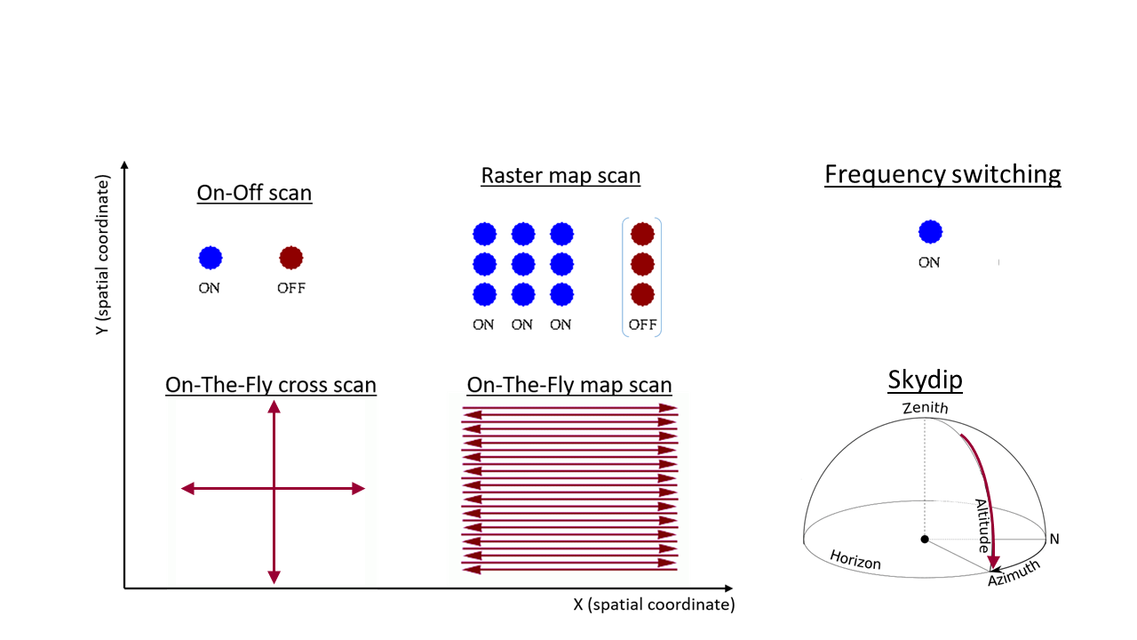
The combination of telescope, frontend and backend permits the realization of various observing strategies characterized by specific spatial and/or spectral patterns. Typical SD observing strategies are: on-source, frequency switching, on-off observations, raster or on-the-fly (OTF) mapping, on-the-fly-cross-scan, skydip calibrations (see Fig ObsCoreExtensionForRadioData:fig:SD). For each spatial position in the observation, SD data gather emission for any of the spectral samples in the given frequency band and polarization. If multi-feed/PAFs are used, a set of spatial positions are simultaneously measured. Scan modes should be described in ObsCore in order to allow astronomers to better understand the structure of the data which will be retrieved.

Spatial resolution in the SD case is intended as the beam size. This holds true for any type of receivers, since also for multi-feed/PAF ones the spatial resolution is ruled by the size of the individual beam.

Contrary to what usually happens for interferometric observations, for some radio telescopes a SD observation (scan) contains only one scientific target (for example INAF ones). In any case, each target in an observation is listed as a separate entry in an ObsCore table sharing the same obs_id.

Complex frequency setups are possible in the same observation, as already mentioned in Sect. 2 Radio data specifities from the Data Discovery point of view.

The ObsCore parameter t_resolution, defined as the minimal interpretable interval between two points along the time axis (being it an average or representative value), has a limited application for SD data except for on-source tracking observations like those for pulsar/FRB studies. Typically, time is not an independent variable in SD measurements and it can be saved together with spatial/spectral/intensity information as a timestamp associated to each data sample. A more comprehensive discussion on ObsCore parameters for time-domain data is given in the Pulsar and FRB Radio Data Discovery and Access IVOA Note [3].

2.2 Visibility data#

Visibility data are sets of complex numbers corresponding to the amplitude and phase of correlation coefficients measured between pair of antennas (i.e., a baseline), at a given time, a given wavelength or polarisation. The visibility data are a sparse representation of the observed sky. The visibility data sets can be processed to obtain interferometric images, through inverse Fourier algorithms. Each visibility measurement corresponds to an interferometric fringe system on the sky.

The imaging algorithms include a calibration step allowing to set the center of the reconstructed image, setting this direction as a phase reference. The visibilities are then usually represented in a spatial frequency plane, called the uv plane, whose orientation is perpendicular to phase reference direction. The instantaneous PSF (Point Spread Function) of an interferometer is the Fourier transform of all baselines sampled in the uv plane. Hence, the quality of the reconstructed images are directly related to the set of baselines used for the measurements.

Visibility data are usually organized as sets of matrices for various phase references (i.e., pointing, or fields) and configuration of the baselines, such as their distances and orientations. Such matrices may or may not be regularly sampled in time, wavelength and polarisation.

As for any other observation product described with ObsCore, the description may be split into several records in the ObsCore table, when ObsCore parameters cannot represent the variety of the observation results coverage (e.g., if there are several observed “fields”, requiring different s_ra and s_dec value, or various groups of spectral bands, etc.)

We consider that consistent ObsCore records as described above define datasets with a dataproduct type set to “visibility”.

Contrary to what occurs with direct imaging observations, the PSF of the interferometer is filtering spatial scales (large scales, when the small baselines are insufficiently sampled; and vice versa for small scales with long baselines). For large spectral ranges, the variations of the field of view and the spatial resolution along the axis may become so large that the typical value cannot be sufficient to characterize the dataset. Ranges of values for such parameters are required to accurately describe such datasets.

The quality of the data strongly depends from the distribution of the visibility measurements in the uv plane : the more complete the uv sampling plane, the better the reconstructed image. The uv plane distribution can be characterized by several numbers. The minimal and maximum distance between measurements in the uv plane provide assessments for spatial resolution and largest angular scale. Beside this a uv plane filling factor of the distribution will allow to predict the quality of reconstruction of the image in the distance plane (sky). Eventually, the ellipticity of the distribution is a measure of the distortions that can affect the reconstruction.

Radio astronomers also check the quality of the visibility data by looking at some maps of the data structure. The uv coverage map can show how complete and regular is the sampling in the uv plane and give an hint of resolution and maximum angular scale. The visualisation of the dirty beam, which is the Fourier transform of the uv sampling function gives an hint of the intrinsic quality of possible reconstruction. As maps they are not queriable. So links to these kind of maps will not be exposed in the extension table but only via a DataLink service.

If none of these uv characterization features are available to be exposed in the service we can still predict ranges of some of those by using parameters of the instrumental configuration. Important features are the antenna diameter (or maximum antenna diameter), the number of antennas and the minimum and maximum distance between antennas of the array.

In addition to these specifities most of the scan modes shown on figure ObsCoreExtensionForRadioData:fig:SD also apply to some interferometry observations and should be described.

3 ObsCore attributes definition valid for radio data#

For radio data some of the definitions on ObsCore data model attributes need to be adjusted to fit the peculiarity of metadata for datasets partition, uv space, etc. Here is a list of common ObsCore parameters already available for the radio data discovery.

3.1 obs_id#

Astronomers usually know what they identify as a single observation: a complex set of measurements made in a given sequence of time. obs_id should define unambiguously each observation. It is provided by the observation pipeline to identify what is collected for one observation operation.

3.2 obs_publisher_did#

Radio data observations can be split in several subparts with homogeneous spatial, time, spectral coverage intervals, spectral resolution, etc. Each part can be described by a single dataset and has its own obs_publisher_did. It has to be unique in the Virtual Observatory domain. It identifies a dataset with homogeneous properties in terms of coverage on all physical axes : temporal, spectral, spatial.

3.3 s_fov#

This attribute measures the size of the field covered. It usually depends on the spectral interval and of the telescope diameter. A typical value for the size of the field of view is to be computed on the observation by taking into account the sky scan geometry and the receiver type in use. s_fov coincides with the instantaneous field of view \(\lambda / D\) only for pointed observations (for instance, an ON in the SD case) obtained with a mono-feed receiver. In this case, \(\lambda\) is the receiver nominal wavelength and D coincides with the telescope diameter (SD case) or the largest diameter of the array antennae or telescopes (interferometric case). In interferometry, the correlator can also restrict the fov depending on the trade-off set to build the signal. Nominal wavelength SHOULD be taken as the mid value of the spectral range except if data providers have good reasons to propose another value which should be documented in the FIELD DESCRIPTION tag in that case.

3.4 s_resolution#

In the case of SD using mono- or multi-feed/PAF receivers this is the beam size inferred from the wavelength and telescope diameter. In the case of interferometry, a typical value for the spatial resolution will be given by \(\lambda / L\) where \(\lambda\) is the receiver nominal wavelength and L is the longest distance in the uv plane. As above nominal wavelength SHOULD be taken as the mid value of the spectral range except if data providers want for specific reasons. For beamforming applied to SD s_resolution is set by the size of one individual electronically-formed beam.

3.5 s_region#

The shape of the covered region. For single dish data it will strongly depend on the scanning mode and type of receiver in use. This shape will be the typical contour of the detectable beam for interferometry. Of course it cannot be accurate.

3.6 o_ucd#

This is UCD string to qualify what is the observable quantity varying along the axes. In the current UCD vocabulary (UCD1+ controlled vocabulary - Updated List of Terms Version 1.5) there appear to be no primary words suitable to describe raw SD data. o_ucd=phot.flux.density does not seem appropriate, since the single dish measured quantity is expressed in raw counts coming from the digitization of a voltage signal generated in the receiver chain by the incoming electromagnetic field. o_ucd=phys.voltage is validated for addition into the next version for UCD1+ controlled vocabulary - Updated List of Terms Version 1.6.

In the case of visibility data the “observable” is a complex number representing Fourier coefficients of the image Fourier transform. Its UCD string is stat.fourier.

3.7 t_exptime#

Total duration of the observation for the given dataset or ObsCore entry. For instance in case of multiple targets, t_exptime will be computed for each source and written in the appropriate ObsCore Table entry. The specific case of time series is addressed in another specification [4].

3.8 t_resolution#

The ObsCore parameter t_resolution (see Sect. 2.1 Single dish data) has a limited application for SD data except for on-source tracking observations like those for pulsar/FRB studies and could be set to the exposure time or could be NULL. For time-domain data, t_resolution can be set according to the Pulsar and FRB Radio Data Discovery and Access IVOA Note [5].

For interferometric observations it is the integration time set at the correlation level.

3.9 dataproduct_type and dataproduct_subtype#

Radio astronomy data cover a wide variety of data product types from visibility for raw interferometry data to cubes, images, spectra, time series or even measurements (in the case of single dish on scan mode). Single dish observations in some modes show specifities which are not covered by the current ObsCore dataproduct_type vocabulary. This is the case of spatial profiles obtained with on the fly cross scan or of the tables of flux measurements obtained on a regular spatial grid but with specific time stamp for each spot as in the raster map mode. A new external standard IVOA vocabulary is currently defined for data product types [6] and tackles some of these specificities. However some of them SHOULD be covered in the dataproduct_subtype attribute if no new term is introduced in the standard vocabulary.

4 ObsCore extension specific for radio data#

Tables ObsCoreExtensionForRadioData:tab:ExtensionAtt, ObsCoreExtensionForRadioData:tab:ExtensionAtt_interferometry and ObsCoreExtensionForRadioData:tab:ExtensionAtt_instrumental show the querying parameters we propose to include into the ObsCore radio extension table in order to better describe radio single dish and visibility data.

4.1 Spatial parameters#

For extended spectral range datasets s_fov_min, s_fov_max are estimated like in the typical value case (see subsection 3.3 s_fov). In the case of SD pointed observations with mono-feed receivers and the majority of interferometric observations the minimum and maximum \(\lambda\) values in the spectral range(s) will be used in the formula \(\lambda / D\) to estimate respectively s_fov_min and s_fov_max.

In the case of mapping scans or multi-feed/PAF receivers s_fov_min and s_fov_max are derived as the minimum and maximum sizes of the circular region encompassing the covered area.

s_resolution_min, s_resolution_max are estimated like the typical value by the formula \(\lambda / L\) (see subsection 3.4 s_resolution) where \(\lambda\) is replaced respectively by the minimum and maximum wavelength of the spectral range(s). The size L is the telescope diameter for SD observations and the largest distance in the uv plane for interferometry. Beam forming may represent an exception to this rule, see 3.4 s_resolution.

In the case of interferometry, we introduce the new s_largest_angular_scale which is estimated as \(\lambda/l\) where \(\lambda\) is the typical wavelength (and again typical value SHOULD be estimated as the mid value of the spectral range apart from documented exceptions) and l is the typical smallest distance in the uv plane. This parameter is not relevant for other observation modes. The largest angular scale is also variable along the spectral range. That’s why we bound it with s_largest_angular_scale_min and s_largest_angular_scale_max estimated as respectively \(\lambda\_min/l\) and \(\lambda\_max/l\)

4.2 Frequency characterization#

As was stated above (2 Radio data specifities from the Data Discovery point of view) radio astronomers use frequency quantities to characterize their datasets. Therefore we introduce one additional parameters in the extension : f_resolution for absolute spectral resolution, which is a more stable parameter than the resolution power in the radio domain.

For users willing to access spectral ranges in frequencies we can imagine several scenarii:

compute two free parameters f_min and f_max this way f_min = c / em_max and f_max = c / em_min with c = 299 792 458 m/s
express queries and results in terms of frequencies by using the same formulae in the ADQL queries (see ObsCoreExtensionForRadioData:sec:FreqRanges)
let the interface do these conversions

Using the ADQL User Defined Functions udf-catalogue in queries for unit conversion as well as ivo_interval_overlaps, ivo_specconv would simplify the interface for the user and avoid columns duplication for the spectral coverage .

4.3 Spatial frequency coverage for visibilities#

These parameters are valid for interferometry only.

The absolute uv_distance_min and uv_distance_max in the uv plane give some outlier minimum and maximum scale in some direction.

To compute the ellipse’s eccentricity of the uv distribution a principal component analysis (PCA) with 2 components is performed over the data points sampling the uv plane to select the main axis of data scattering. The first component is used to rotate the distribution of uv in a way that the major variation of the distribution is leaning towards the \(x\) axis of a bi dimensional \(xy\) Cartesian plane. The major axis length and the minor axis length of the ellipse are therefore defined as the semi distance between the most positive point along the \(x\)/\(y\) axis and the most negative point among the \(y\) axis. For instance, if the range of the rotated UV will cover on the \(x \in [-10, 10]\) the major axis distance would be 10, a similar procedure is done on the y axis.

This procedure allows the definition of the uv distribution eccentricity, uv_distribution_ecc computed as follows:

\[\begin{equation} uv\_distribution\_ecc = \sqrt{1-\frac{b^2}{a^2}} \end{equation}\]

where a is the major axis length and b is the minor axis length. The filling factor of the uv plane (hereafter uv_distribution_fill) is computed as the average number of samples found in a \(N^{uv}_{samples}\)x\(N^{uv}_{samples}\) equi-spaced grid enclosing the rotated ellipse. In formulas, the boundaries of a cell (i,j) are defined by the boundaries

\[\begin{equation} u \in [u_{min} + \frac{u_{max} - u_{min}}{N^{uv}_{samples}} \cdot i , u_{min} + \frac{u_{max} - u_{min}}{N^{uv}_{samples}} \cdot (i + 1)] \end{equation}\]

and

\[\begin{equation} v \in [v_{min} + \frac{v_{max} - v_{min}}{N^{uv}_{samples}} \cdot j , v_{min} + \frac{v_{max} - v_{min}}{N^{uv}_{samples}} \cdot (j + 1)] \end{equation}\]

where \(u_{max}\)/\(v_{max}\) are the respective maximum u/v of the uv sample and \(u_{min}\)/\(v_{min}\) is the minimum u/v of the uv sample.

Given the above boundaries the number of samples within a cell (i,j) will be \(n^{uv}_{i,j}\) and uv_distribution_fill will be then computed as

\[\begin{equation} uv\_distribution\_fill = \frac{\sum^{N^{uv}_{samples}}_{i=1} \sum^{N^{uv}_{samples}}_{j=1} n^{uv}_{i,j} }{(N^{uv}_{samples}) ^ 2}, \end{equation}\]

in the preliminary analysis \(N^{uv}_{samples} = 1000\).

4.4 Observational configuration and instrumental parameters#

These parameters are intended to describe the main telescope(s) characteristics for both SD antennas and interferometers. Such instrumental characteristics give an approximate idea on the spanned angular scales, field of view, product types, etc.

The more global parameter to define is the instrument type allowing to discriminate single dish observations from interferometry or beam forming ones.

Parameters instr_tel_number, instr_tel_min_dist and instr_tel_max_dist are related to interferometers only while instr_tel_diameter, instr_feed are valid also for SD. We note that instr_feed could also account for the number of beams in the case of a beam forming/PAF receiver.

The scanning strategy adopted in an observation is described by the parameter scan_mode. This parameter covers both spatial and frequency scanning modes (see Sect. 2.1 Single dish data for details and table ObsCoreExtensionForRadioData:tab:scanmode for possible values). It is applicable to SD as well as to interferometry cases.

Pointing mode distinguishes observations pointed on a fixed target from observations fixed on a given elevation and azimuth. The ObsLocTAP specification ObsLocTAP defines the term tracking_type for describing this as well as a vocabulary for these modes. We include the same terms here in the present extension. The possible values for radio astronomy data are the following:

sidereal : observations pointed on a fixed target, as defined in ObsLocTAP
fixed-az-el-transit : observations fixed on a given elevation and azimuth, as in ObsLocTAP
Solar-system-object-tracking : moving target, like moon or solar bodies

4.5 Auxiliary datasets for data quality estimation#

Auxiliary datasets such as uv distribution map, dirty beam maps, frequency/amplitude plots, phase/amplitude plots are useful for astronomers to check data quality.

In that case, DataLink DataLink may provide a solution to attach these auxiliary data files to ObsCore records. The link between a data set and its associated data files, is described by a set of parameters in the specification as shown in the datalink table example below.

5 The ivoa.obscore_radio table#

The ObsCore Extension for Radio is accessed as a table within a TAP TAP service. At this point, the name of this table is fixed to ivoa.obscore_radio. Within the IVOA, it is forbidden to use this name for anything else than a table compliant with this specification.

A TAP service that has ivoa.obscore_radio must also have a table compliant to any version 1 of ObsCore, i.e., a table ivoa.obscore containing only the basic ObsCore attributes. The two tables must share exactly the obs_publisher_did column such that a NATURAL JOIN will yield per-dataset rows of obscore and radio extension metadata.

To ensure that all compliant services can execute the same queries, all columns described in following tables ObsCoreExtensionForRadioData:tab:ExtensionAtt , ObsCoreExtensionForRadioData:tab:ExtensionAtt_interferometry and ObsCoreExtensionForRadioData:tab:ExtensionAtt_instrumental must be gathered in the ivoa.obscore_radio table, although some of them may be NULL if no value apply . At least a foreign key into ivoa.obscore will typically make the extension table user-visible.

The intention is that clients will write queries like

SELECT [any obscore and obscore_radio columns or expressions]
FROM  ivoa.obscore
NATURAL JOIN ivoa.obscore_radio
WHERE [constraints]

6 Registry Aspects#

Services compliant with this specification are registered using VODataService VODataService tablesets. Compliant tables use the utype

\[\hbox{\nolinkurl{ivo://ivoa.net/std/ObsCore#radioExt-1.0}.}\]

While it is admitted that the table only sits in the tableset of the embedding TAP service, implementors are urged to use a separate registry record with the main TAP service as an auxiliary capability [discovercollections1.1]. In this way, meaningful information on coverage in space, time, and spectral axes as per VODataService 1.2 can be communicated to the Registry, which data providers are urged to do.

However, discovering the obscore_radio table alone would be irrelevant. The same service delivering the obscore_radio table MUST also contain the ObsCore table. Being sure our service contains these both tables, the user is able to build any natural JOIN query between these two tables.

To obtain access URLs of all TAP services that have compliant tables together with their table names (which in this major version are fixed to ivoa.obscore_radio), use a RegTAP [RegTAP1.1] query like:

SELECT DISTINCT(access_url), table_name
FROM rr.res_table
  NATURAL JOIN rr.capability
  NATURAL JOIN rr.interface
WHERE
  standard_id LIKE 'ivo://ivoa.net/std/tap%'
  AND intf_role='std'
  AND table_utype LIKE 'ivo://ivoa.net/std/ObsCore#radioExt-1.%'
  AND EXISTS (select 1 from rr.res_table where
                table_name LIKE '%obscore')

In the current status of the ObsCore specification the last statement in the WHERE clause is the simplest one to ensure the service also delivers the main obscore table. In the future this statement could be replaced by

AND EXISTS (select 1 from rr.res_table where
   table_utype LIKE 'ivo://ivoa.net/std/obscore#core-1.%')

When we will have other extensions (for example for time series or high energy data) we may want to discover services supporting several extensions in addition to the ObsCore main table.

Searching ObsTAP services with multiple extensions could be done by a query to the relational registry such as:

SELECT DISTINCT(access_url), table_name
FROM rr.res_table
  NATURAL JOIN rr.capability
  NATURAL JOIN rr.interface
WHERE
  standard_id LIKE 'ivo://ivoa.net/std/tap%'
  AND intf_role='std'
  AND table_utype LIKE 'ivo://ivoa.net/std/ObsCore#radioExt-1.%'
  AND EXISTS (select 1 from rr.res_table where
       table_utype LIKE 'ivo://ivoa.net/std/ObsCore#timeExt-1.0'
  AND EXISTS (select 1 from rr.res_table where
    table_name LIKE '%obscore')

assuming that the standardID for the time extension currently in progress will be

\[\hbox{\nolinkurl{ivo://ivoa.net/std/ObsCore#timeExt-1.0}}\]

In addition the tableset schema containing the ObsCore main table and potentially some of the extensions SHOULD use the root ObsCore standardID utype :

\[\hbox{\nolinkurl{ivo://ivoa.net/std/ObsCore}}\]

Then the following query would allow to discover all services exposing ObsCore metadata as well as the extension tables they deliver.

SELECT DISTINCT(access_url), table_name, schema_name
FROM rr.res_table
NATURAL JOIN rr.capability
NATURAL JOIN rr.interface
NATURAL JOIN rr.res_schema
WHERE
standard_id LIKE 'ivo://ivoa.net/std/tap%'
AND intf_role='std'
AND schema_utype LIKE 'ivo://ivoa.net/std/ObsCore'