MOC: Multi-Order Coverage map#

Status:: moc 2.0 REC 2022-07-27

Acknowledgments#

This work has been supported by the ESCAPE project (the European Science Cluster of Astronomy & Particle Physics ESFRI Research Infrastructures) that has received funding from the European Union’s Horizon 2020 research and innovation Programme under the Grant Agreement n. 824064.

1 Introduction#

This document is a major release of the already existing encoding method recommendation Multi-Order Coverage map citep[MOC~1.1,][]{2019ivoa.spec.1007F}. We generalize the MOC originally limited to space dimension (Space MOC, SMOC) to the time dimension (Time MOC, TMOC), and space and time dimensions (Space-Time MOC, STMOC). Figure moc:fig:ivoadiagram illustrates the role MOC2.0 plays within the IVOA architecture [IVOAArchitecture2.0].

The encoding method described in this document allows one to define and manipulate space and time coverage in such a way that basic operations like union, intersection, equality test can be performed very efficiently. This methodology allows VO applications and data servers to build efficient procedures to perform such operations on observations and catalogs. In the next sections we will describe the different MOCs and their encoding standards.

2 The rationale#

The goal behind the MOC is to get a method to manipulate coverages in order to provide very fast union, intersection and equality operations between them. In order to accomplish this task, we based the system on a regular and hierarchical discretization as exposed below. The standard MOC1.0 was limited to space, but for a multitude of use cases in astronomy we need the notion of time to be properly integrated, e. g.:

What are the space and time coverages of the 2MASS observations and are there any observations which are coincidental with the HST archive?
Which are the astronomical catalogs which have data for a list of Supernova events within a given time window?
Are there any other observations coincidental with this gravitational wave detection given its time and spatial coordinates?
Are there quasi-simultaneous observations (within a given time window) of these two surveys for a list of eclipsing binaries?
Find the intersection between the SDSS coverage and the ephemeris of this Near Earth Object, was it observed by SDSS? And by Galex? By both missions simultaneously? If so, are there detections within the source catalogues?
Has Neptune been observed by DSS?

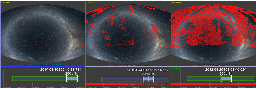
It was possible to answer those questions with MOC1.0 standard and other VO tools but the amount of manipulation and computation was quite a big hurdle for the researchers. With MOC2.0 it is possible to answer these questions in a few milli-seconds. Another example of usage would be the visual inspection of the spatio-temporal coverage of PanSTARRS observations (see Figure moc:fig:panstarrs). The choice of a temporal resolution and a spatial resolution makes it possible to obtain a MOC of a desired data volume.

2.1 Comparing the coverage of multiple data sets#

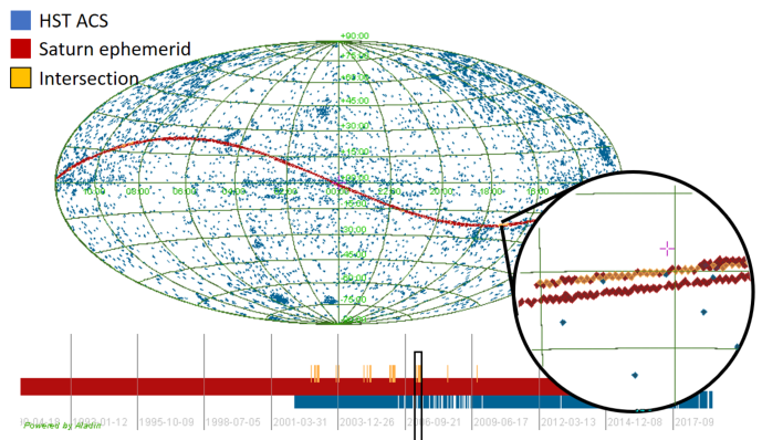
The computation of data set intersections using the MOCs is simple (it is simply a list comparison). The result of any operation is itself a MOC which can be used in further operations. For instance it is possible to compute the intersection of Saturn’s ephemeris and the spatio-temporal coverage of HST ACS observations, and subsequently, query a database for retrieving images for which time and position fall within this intersection (see Fig. moc:fig:stmoc-saturn).

2.2 Query databases using MOC#

In principle, querying a positional database using complex sky region coverage is possible using ADQL. However, this is rarely possible when the sky region has to be described as unions and intersections of sub-regions to cover a complex, non regular area. In practice, most existing ADQL implementations only support simple regions (cones, boxes, polygons), and can rarely deal with unions and intersections unless by joining independent queries – and this even if the described region is, in fact, empty! If databases are adapted to supporting MOC based queries, they will offer then a useful method allowing any kind of sky region query. In addition, if the internal spatial index of the database is itself based on HEALPix, the filtering will then be straightforward and all the intermediate sky computations will be removed providing an optimal response time.

2.3 Gravitational Wave localisations#

The contours of a gravitational-wave sky localization are constructed as follows. The pixels from most probable to least are ranked, and summed up to get a fixed level of probability []. In practice, the HEALPix pixels inside a given contour plot are extracted, and the MOC coverage is generated from the table made up from the pixels. Every single level of probability can be used as a regular MOC even in the case in which the sky localization is irregularly shaped with disjoint regions. This coding technique allows for an extra fast integration in the existing Virtual Observatory structures and tools [1]. The 2D contours of a GW sky localization can be visualised and manipulated using Aladin Desktop, allowing one to compare them with existing surveys, overlap sky map generations with increasing accuracy and computational cost and query the VizieR database. These sets of tasks can also be performed via Python using the astropy affiliated package mocpy [2], efficiently displayed in javascript applications with Aladin Lite, and integrated within Jupyter notebooks through the ipyaladin widget [3].

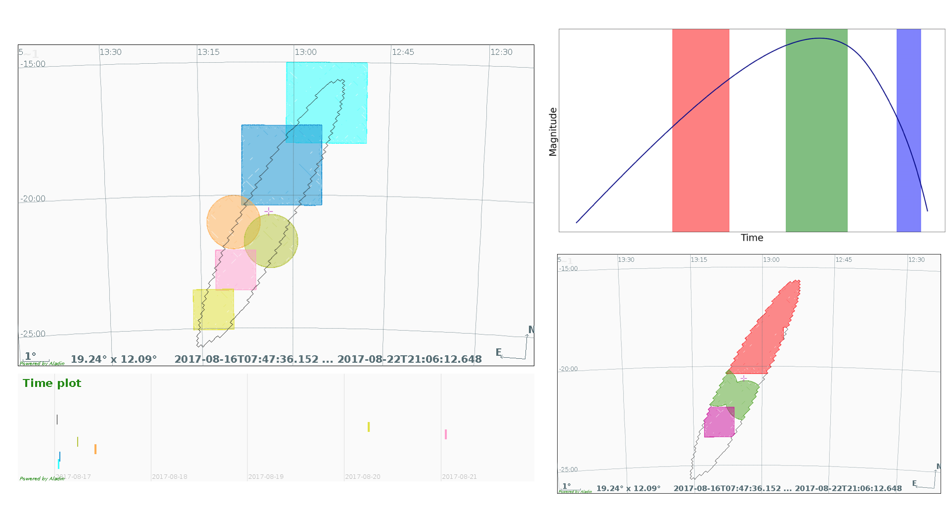
Adding temporal information in a space MOC encoding can provide a systematic approach in extracting information from follow-up campaigns involving tens of ground and space-based observatories in searching for gravitational-wave counterparts. For illustrative purposes only, a potential use of the time-space MOC is provided when a kilo/macronova emission is a credible counterpart of a gravitational-wave event. Figure moc:fig:gw shows a mock electromagnetic follow-up campaign of a gravitational-wave sky localization over a period of time (left panel), a schematic kilonova light-curve and temporal coverage of observations (top right panel) and associated spatial coverage (bottom right panel). This approach permits us to depict the approximate timeline of the instruments involved in the observational campaign and place constraints on the emission properties during the source evolution.

2.4 Space and Time MOC: Einstein Telescope and Early Warning Alerts#

The space and time MOC provides us with an effective way to develop new multi-messenger data analysis tools that will have a crucial role when the third-generation interferometric gravitational wave observatories, such as the Einstein Telescope (ET), will begin operation. Here we figure out a few potential applications. ET will explore the universe with gravitational waves up to cosmological distances with an expected detection rate of order \(10^{5} - 10^{6}\) black holes and \(7\times10^4\) neutron star mergers per year []. For fast and real time data access, the user can query by a specific time range the gravitational-wave sky localizations encoded as a space and time MOC.

In addition, the ET sensitivity at low frequencies enables enough signal-to-noise ratio to accumulate before the merger, making possible a pre-merger gravitational-wave detection and warning for the electromagnetic/neutrino follow up. The simulations show that, by requiring a signal-to-noise ratio \(>=\) 12 and a sky localization smaller than 100 deg\(^2\), ET can send an early warning alert between 1 and 20 hours before the merger (with the mean of the distribution at about 5 hours) for signals at 40 Mpc []. The electromagnetic/neutrino survey can benefit in multiple spatial and temporal intersections with a gravitational-wave sky localization to probe any electromagnetic/neutrino signals temporally and spatially connected to the inspiral, merger or ring-down phases. Early warning alerts are also planned in the LIGO-Virgo-KAGRA O4 run with an experimental capability to produce and distribute early warning gravitational-wave alerts up to tens of seconds before merger [4].

2.5 Multi-site positional and temporal search#

Often, a typical query from a virtual observatory (VO) user is to request all possible records from the VO at a given sky position and/or at a given time. While this is in principle possible by dispatching one narrow positional query to every registered Cone Search, SSA or SIA service and filtering by time, in practice, the number of queries required leads to an unacceptable load on both clients and services. Moreover, most of these queries will deliver no results since most services often lack coverage in the queried region. If basic footprint/coverage information was available for all registered services, for instance using VODataService 1.2 VODataService only those with coverage in the region and time of interest would then be queried. This would provide a great reduction in the number of services to be queried optimizing the response time. Using the MOC offers the opportunity to provide this coverage information in a uniform way. The MOC could be stored locally for a given service or centrally where the coverage for a number of services would be supported.

3 MOC principles#

The MOC standard is defined using four basic building blocks: discretization, unique reference system, hierarchization and efficient encoding:

Determine a proper tessellation/discretization methodology for each dimension axis (space, time, …);
Fix a unique referential system for each dimension, to avoid reference conversions and thus allowing to easily compare different data collections;
Use an hierarchical procedure and a unique representation (canonical form) for compacting and quickly manipulating each axis coverage at any level of accuracy;
Implement at least one serialization in a binary encoding format (other serializations are possible, e.g. ASCII).

With these principles, a MOC consists of a list of numbers which represent the indices of the cells mapping the coverage of the spatial or temporal axis. As soon as the consecutive cells are used at order n, they will be hierarchically grouped in their parent cell at order n-1, and this recursively. This introduces the notion of orders and associated cell index. The cell boundary alignment implied by the hierarchical structure facilitates the combination of cells at different orders. To work efficiently on existing hardware, we encode of any pair (order, index) as a long integer (64 bits), and we reserve the two most significant bits to encode the type of MOC (spatial, temporal, or future usages). The earlier MOC standard was limited to spatial coverage. We are reusing these principles to manipulate temporal coverages, as well as space-time coverages where we can manipulate the two physical dimensions simultaneously.

We will now explain the conventions chosen for the spatial and temporal axis.

3.1 Space MOC conventions#

Defining a sky region by a subset of regular sky tessellation or tiles is not a new idea. In astronomy, one could find three main methods of partitioning the sphere : Q3C, HTM and HEALPix which are respectively using cells in the form of squares, triangles and diamonds for mapping the celestial sphere.

Several publications have compared these methods []. We justified the choice of HEALPix for the MOC because of these four points:

Equal areas: by construction, HEALPix consists of diamond cells with equal spherical surfaces. Thus the area of a given region is trivial to compute;
Computing time: HEALPix has the peculiarity that the computing time does not depend on the hierarchical order [5] (no recursive algorithm);
Accuracy: HEALPix provides libraries which allow the calculation up to accuracy of 0.4 mas (order 29) (http://sourceforge.net/projects/healpix/);
Standard: Existence of many HEALPix libraries: C++, Java, Fortran, IDL… Also, HEALPix was selected for several all sky missions such as WMAP, Planck and Gaia. The HEALPix main web site is located at Jet Propulsion Lab (http://healpix.sourceforge.io/).

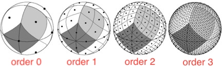
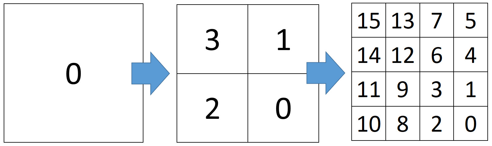
The HEALPix [] tessellation technique divides the sphere into 12 cells, each of them sub-divided into 4 cells recursively (see Fig. moc:fig:healpix). Thus the sphere at order 1 will consist of 48 cells, 192 cells at order 2, 768 at order 3 and so on where each cell at a given order is covering an equal area of the sphere.

HEALPix allows three coordinate systems: galactic, equatorial and ecliptic. Allowing various coordinate systems would limit the possibility to compare efficiently SMOCs. There is indeed no equivalence between an HEALPix cell described in a given coordinate system and a cell, or a list of sub-cells expressed in a different coordinate system. Consequently, the SMOC definition is expressed in equatorial coordinate using the ICRS reference. This choice has been motivated by looking at most catalogs and realizing that most of them are using equatorial coordinates.

To support the encoding based on 64-bit longs, the best resolution available is provided at order 29 and according to the HEALPix equations, corresponds approximately to 0.4mas. The SMOC resolution is set by the maximum value of the HEALPix order used to define a region. Its selection depends on the accuracy chosen by the provider to define the region. As data set boundaries are not aligned with the HEALPix cell borders, a SMOC is generally an upper-approximation of the data set coverage. The quality of this approximation depends directly on the chosen SMOC resolution (MOCORD_S). Table moc:table:orders provides the HEALPix cell angular resolution for each HEALPix order.

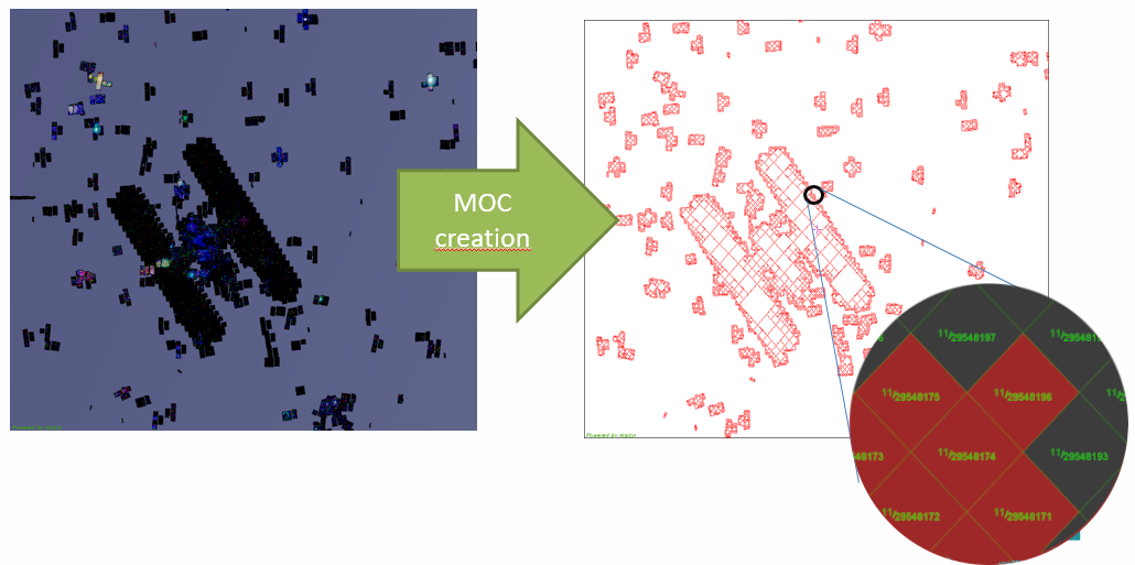
In Figure moc:fig:smoc-view we show the MOC creation, from images to their coverage, and indicating their corresponding HEALPix numbers.

3.2 Time MOC conventions#

In order to represent time coverage, we need to select a-priori the total range of time that we will cover with the notation. Following the same SMOC principles, we need to use a discrete time axis where each unit element of this axis has a constant duration. We adopt the Julian Date convention, very common in astronomy and a nominal resolution of 1\(\mu\)s. The temporal dimension being by nature 1D unlike the spatial dimension, we opt for a order progression by factor of 2 (4 for SMOC) and therefore 62 orders (30 for SMOC). This way we can address \(2^{62}\) cells in an unsigned 64-bit integer, i.e. a little bit more than 73000 years at 1\(\mu\)s resolution, enough for most astronomical time events. At the deepest order (61) the TMOC cell number is the number of \(\mu\)s since JD=0.

The time is a relative observation, and depends on the position of the observer. There are many time scales for measuring time: Terrestrial Time (TT), Barycentric Coordinate Time (TCB), Geocentric Coordinate Time (TCG), Ephemeris Time (ET), Barycentric Dynamic Time (TDB), International Atomic Time (AI), etc. We opt for the TCB reference (see cite{2015A&A…574A..36R} for details). Our choice is motivated by the fact that this system is linear by construction and has been adopted by numerous missions such as Gaia.

It may be necessary to convert the temporal events to the chosen scale. If the ephemeris required for this conversion are not available, opt to degrade the accuracy of the time measurement (typically around 20 minutes for observations within the Earth orbit environment to cover all possible observer positions). Table moc:table:tmocorders is showing some time values at a given order.

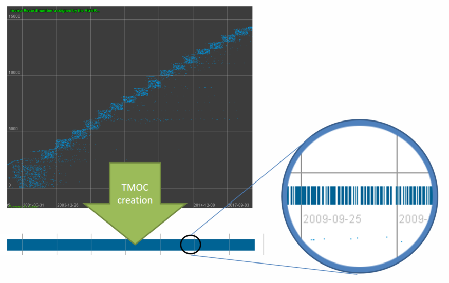
In Figure moc:fig:tmoc-view we show the creation of TMOC, from a time series to the list of numbers based on time discretization.

3.3 Space and Time MOC conventions#

To respond to the different use cases presented at the beginning of the document, the SMOC and TMOC independently are not enough. We need to link the two dimensions in a global mechanism. In other words, we need to be able to select the SMOC using a time window or to select a TMOC using a spatial constraint. Implementing this linkage would allow the potential users to select and interact with the astronomical collections which support space and time and use logical operators between them.

Our approach is to combine these two dimensions - time and space - by associating each time period (coded according to the TMOC convention) with its spatial region (coded according to the SMOC convention). For that, we interleave the information of time coverage with the information of space coverage for this period.

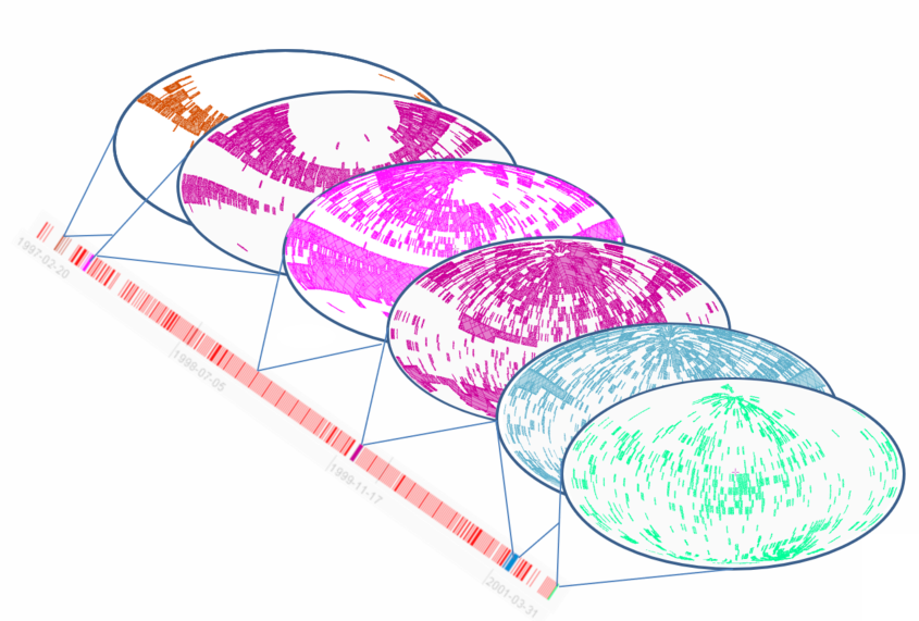
This two-dimensional interleaving approach has the advantage of making the resolutions chosen for time and for space independent. For instance, it is possible to describe observation coverage with a low resolution for time while using a high spatial resolution. A single coding for indexing space and time simultaneously would imply at best very low resolution MOCs due to the 64-bit coding constraint. We thus proposed the interleaving algorithm which allows us to define and manipulate high resolution STMOCs of reasonable sizes for fast algorithms (see Appendix moc:app:perf for STMOC performance). In Figure moc:fig:stmoc-view we show the visual representation of an STMOC, in which at a given TMOC range we obtain the corresponding SMOC.

4 SMOC and TMOC encoding#

The encoding described in this section guarantees backward compatibility with MOCs corresponding to previous versions of this standard.

4.1 Space MOC or SMOC#

As introduced above, the SMOC should be based on the HEALPix tessellation of the sphere, expressed in the ICRS coordinate reference system for celestial coverages. This document does not describe the use of SMOC outside celestial scope. However, it is possible to use SMOC for other coverages, such as planetary coverages. The definition of the unique reference for each body will have to be defined. Two complementary encoding formats are defined: a string serialization based on ASCII and a binary format based on FITS.

4.1.1 Numbering#

The numbering scheme used in SMOC for specifying the cell indices must follow the “NESTED” HEALPix numbering schemes []. This numbering consists of enumerating all cells in a specific order. For instance, at order 1, there are 48 cells (12x4) enumerated from 0 to 47. In this scheme, the 4 sub-cells of cell M have the indices: (M\(\times4)+3\), (M\(\times4)+1\), (M\(\times4)+2\), (M\(\times4\)) in reading order. And reciprocally, the parent index of cell N is N/4. Each SMOC cell is coded by a pair of numbers: (order, index) which are the HEALPix order and the HEALPix index in this order.

Note: The order 0 is a special case, it contains only 12 cells enumerated from 0 to 11.

4.1.2 Sky coordinates#

The mechanism used to determine which HEALPix cell contains a given sky location is described in the main article defining the HEALPix system []. Several support libraries supporting the most important set of primitives are already available. These libraries are required if one wants to generate SMOCs, and also wants to compare them with sky coordinates. Though please note that these libraries do not have built-in support to performing basic SMOC arithmetics.

4.2 Time MOC or TMOC#

As introduced above, TMOC must be based on JD system, the time scale TCB, and the Solar System Barycenter as the reference position citep[see also][]{2019ASPC..523..497F} and section 3.2 Time MOC conventions. The best resolution supported by TMOC is \(1 \mu\)s.

In the case that the time scale and the time reference position are unknown, we recommend to set the time resolution of the generated TMOC to order 31, e.g. about 1000 seconds (see Table moc:table:tmocorders) corresponding to about twice the light travel time correction between the Earth and the Solar Barycenter. Please refer to the VO note on TIMESYS for more information about this limitation [].

4.2.1 Numbering#

The numbering scheme used in TMOC for specifying the time cell indices must reuse a similar hierarchical principle as for the SMOC with the difference that the time line has only one dimension, so the hierarchical progression uses a factor of 2 instead of 4, and there is no need to use a HEALPix mapping.

TMOC has 62 orders, and at the best resolution (order 61), a time event will be coded by the integer value representing the number of \(\mu\)s of this event since JD=0.

Two consecutive cells at order N with the indices (M\(\times\)2)+1, (M\(\times\)2) will be coded at order N-1 with the index M and thus recursively. The order N-1 cell duration is 2 times more than the N cell duration (61: 1 \(\mu\)s, 60: 2 \(\mu\)s, 59: 4 \(\mu\)s, etc…).

4.3 Serialization#

A MOC can be manipulated and serialized either as a list of cell numbers for each order (hierarchical view), or as a list of intervals at the deepest order (range view). These two methods are used for SMOC, TMOC and STMOC serializations and are presented below.

4.3.1 Binary serialization#

To encode a MOC in a FITS file, each MOC pair (order, index) must be stored in a FITS binary table. Two packaging modes are defined: either all MOC pairs (order, index) are stored individually thanks to NUNIQ packaging, or all ranges of indices at the deepest order are stored following the RANGE packaging.

NUNIQ Packaging (valid for SMOC only)#

The NUNIQ scheme defines an algorithm for packaging a MOC pair (order, index) into a single integer for compactness:

\[\textit{uniq} = 4 \cdot (4\,^\textit{order}) + \textit{index}\]

The inverse operation is:

\[\begin{split}\begin{eqnarray*} \textit{order} & = &\log_2(\textit{uniq}/4)/2\\ \textit{index} & = &\textit{uniq} - 4 \cdot (4\,^\textit{order}) \end{eqnarray*}\end{split}\]

The list of cells must be well-formed (see Section 7.1 Canonical form) allowing to express both hierarchy or range representation. The resulting list is stored in a single-column binary table extension. For orders strictly lower than 14 these UNIQ values can be stored in a 32-bit signed integer (TFORM1=’J’) , and for the higher orders in a 64-bit signed integer (TFORM1=’K’).

RANGE packaging#

For the coding of RANGE alternative packaging, all the indices are expressed at the maximum resolution, and it is the succession of intervals that will be stored in the FITS table as two 64-bit signed integers (TFORM1=’K’) : the smallest index of the interval and the index strictly greater than the largest value of the interval. The RANGE values must be in ascending numerical order. The resulting list is stored in a single-column binary table extension.

Backward compatibility#

RANGE packaging has been introduced for MOC2.0. This method is generally faster than the previous one for reading or writing a MOC because the internal representation of MOC in memory is often range oriented. However, we recommend to use the first method for SMOC for compatibility with existing libraries not yet compatible with MOC2.0.

4.3.2 ASCII serialization#

To encode a MOC as a string each MOC pair (order, index) must be written sequentially in an ASCII stream as two ASCII numbers separated by slash (“/”: decimal ASCII code 47). The order and the slash prefix may be omitted if the previous cell has the same order. The elements are separated by one or several space characters (space, CR, LF) corresponding respectively to the decimal ASCII codes: 32, 13, and 10.

The usage of a range operator is allowed in the list of indices using the dash (“-”: decimal ASCII code 45) as a separator: lowindex-highindex. The list of cells must be well-formed, and the values must be in ascending numerical order.

If the best resolution of the MOC (moc order) is greater than the greatest stored order, the moc order must be provided, followed by a slash (“/”) without any associated index value. In the following example all the cells underneath the explicit pair (order, cell) are implicitly covered up to order 8, the moc order, annotated followed by the terminator “/”. Without the terminator we would only have the information of the explicit pair (order, cell), and the assumed best resolution would be at order 2.

Example of an ASCII MOC:#

1/1 2 4 2/12-14 21 23 25 8/

	1/1	2	4	2/12-14	21	23	25	8/
	\(\downarrow\)	\(\downarrow\)	\(\downarrow\)	\(\downarrow\)	\(\downarrow\)	\(\downarrow\)	\(\downarrow\)	\(\downarrow\)
Order:	1	1	1	2	2	2	2	8
Cell:	1	2	4	12 to 14	21	23	25

MOC ASCII encoding

EBNF definition of an ASCII MOC:#

smoc  ::= 's'? moc
  tmoc  ::= 't'? moc
  stmoc ::= ('t' moc 's' moc)+
  moc ::= ordval (sep+ ordval)* [sep+ order]
  ordval ::= order sep* vals
  order ::= int '/'
  vals ::= val (sep+ val)*
  val ::= int | (int '-' int)
  sep ::= [ \n\r]
  int ::= [0-9]+

Note that we use Extended BNF supporting regular expression syntax with the following rules: i) postfix * means “repeated 0 or more times”; ii) postfix + means “repeated 1 or more times”; iii) postfix ? means “0 or 1 times”. The first three rules depend on the MOC type, i.e. SMOC for space, TMOC for time and STMOC for space-time.

5 STMOC encoding#

Coding STMOC consists in the following: for each element of a temporal coverage we list the associated spatial coverage using the natural packaging as defined in the previous section.

5.1 ASCII Serialization#

The ASCII serialization of a STMOC is a string following the ASCII MOC serialization presented below, which interleaves time coverage as a excerpt of TMOC and associated space coverage as a SMOC. Each TMOC element must be prefixed by the character ’t’, and each SMOC element must be prefixed by the character ’s’. The character is thus omitted until the next dimension element is defined.

Example of an ASCII STMOC:#

t61/1 s29/0-2 t61/3 s28/0 t60/2 61/6 s29/2 5

	t61/1	s29/0-2	t61/3	s28/0	t60/2	61/6	s29/2	5
	\(\downarrow\)	\(\downarrow\)	\(\downarrow\)	\(\downarrow\)	\(\downarrow\)	\(\downarrow\)	\(\downarrow\)	\(\downarrow\)
Dimension:	Time	Space	Time	Space	Time	(Time)	Space	(Space)
Order:	61	29	61	28	60	61	29
Cell:	1	0 to 2	3	0	2	6	2	5

STMOC ASCII encoding: two independent numbering. Values in parenthesis are implicit from the previous encoding substring.

5.2 Binary Serialization#

The binary serialization of a STMOC is a FITS binary table following the RANGE packaging presented previously, which interleaves time range(s) and their corresponding space coverage ranges. Following the binary RANGE serialization method described below, each range (time or space) is coded as two 64-bit signed integers ([min..max[). To distinguish time and space indices, the time indices must have the 64th bits forced to 1. It is not a sign inversion (two’s complement) but a mask affecting only that last bit without touching any other bits. The order of dimensions is always time first.

Illustration of STMOC interleaving method#

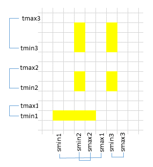
This list of ranges will be coded in a list of 64bits integers (time indices with the 64th bit forced to 1) as:

tmin1 tmax1 smin1 smax1 tmin2 tmax2 tmin3 tmax3 smin2 smax2 smin3 smax3

STMOC encoding must conform to the following simple rules:

Temporal cells which are sequential and have the SAME spatial coverage MUST be aggregated in the coding scheme.
The cell order MUST also be increasing first on the temporal axis, then on the spatial axis.

This is illustrated in Figure moc:fig:stmocbin-encoding.

6 FITS keywords#

For the binary representations which are packaged in binary FITS table, we define a set of FITS keywords, their possible values and set when those fields are required, optional or recommended in Table moc:table:fits_stmoc and show an example of FITS headers for a MOC. Since MOC 1.1 [MOC1.1] the PIXTYPE = "HEALPIX" keyword/value is no longer required, and should be omitted. The keyword MOCORDER is no longer required either, but it can be used for backwards compatibility if required. Other FITS Keywords could be used to augment the information like DATES and ORIGIN.

Example of FITS headers for a MOC:#

SIMPLE   =                      T
BITPIX   =                      8
NAXIS    =                      0
EXTEND   =                      T
END

XTENSION = 'BINTABLE'            / HEALPix Multi Order Coverage map
BITPIX   =                      8
NAXIS    =                      2
NAXIS1   =                      4
NAXIS2   =                  16461
PCOUNT   =                      0
GCOUNT   =                      1
TFIELDS  =                      1
TFORM1   = '1J      '
TTYPE1   = 'UNIQ    '            / HEALPix UNIQ pixel number
ORDERING = 'NUNIQ   '            / NUNIQ coding method
COORDSYS = 'C       '            / ICRS reference frame
MOCDIM   = 'SPACE   '            / Physical dimension
MOCORD_S =                    12 / MOC resolution (best order)
MOCTOOL  = 'Aladin11.1'          / Name of the MOC generator
MOCTYPE  = 'CATALOG '            / Source type (IMAGE or CATALOG)
MOCID    = 'ivo://CDS/I/259'     / Identifier of the collection
MOCVERS  = '2.0     '            / MOC standard version
ORIGIN   = 'ivo://CDS'           / MOC origin
DATE     = '2013-06-15T11:50:43' / MOC creation date
EXTNAME  = 'Tycho MOC'           / MOC name
END

7 MOC usage constraints#

7.1 Canonical form#

The speed of MOC operations - creation, union, intersection, etc is directly dependent on the speed of the equality test. It is therefore essential to always express a MOC in a canonical way, ie one unique representation for one coverage. Thus in the case of a hierarchical representation a MOC must be “well-formed”, i.e. redundant cells are not allowed, the cells must be ascending sorted and the hierarchical encoding principle must be respected. Thus it is not allowed to encode sibling cells instead of their parent (4 siblings for SMOC, 2 siblings for TMOC). In the case of range representation, the list of ranges must be expressed without overlapping and sorted ascending.

7.2 Compromise of Volume VS. Resolution#

In order to easily handle MOCs, it is recommended to adjust the maximum resolution, i.e. the deepest order, to obtain a representation of the desired data volume even if it means degrading the accuracy of the coverage (see Appendix moc:app:perf). In the case of STMOC, it is possible to adjust the spatial order and/or on the temporal order independently.

7.3 Working resolution#

The MOC has been designed to be able to efficiently handle observation coverages (images, catalogs, …). During the construction of the MOC, we must then ensure that at the chosen nominal resolution, any cell of the MOC contains at least one observation (no empty cell). To keep this assumption, during operations (unions, intersections …) between 2 or more MOCs (e.g: MocA \(\cup\) MocB \(\cup\) MocC) of different resolutions, the operations must always be done at the worst (lowest) resolution of the original MOCs in order not to lose any observations, nor to create empty cells (see Figure moc:fig:operation), and finally to guarantee the set logical properties (commutativity, associativity,…).

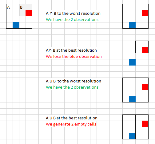
Note that MOC usage can be diverted to also manipulate surfaces unrelated to observations. When it is used this way such operations (oversampling, surface dilatation or surface erosion) can be applied. And in this context it is necessary to work at the best (highest) resolution of the involved MOCs for preserving the properties of the surfaces operations (commutativity, associativity, …).

8 Summary and conclusion#

We have reviewed the standards for encoding the different MOC flavors, the space MOC (already described in version 1.1 of this document), SMOC, the time MOC, TMOC and the space-time MOC, STMOC. The conventions for space and time MOC are the following:

The SMOC is simply defined as a list of HEALPix indices (order, index).
According to HEALPix, the sphere is divided in cells, hierarchically grouped 4 by 4 with 30 orders and the space coverage for the deepest order is approximatively 0.4mas.
The space reference system is ICRS.
The TMOC is simply a list of time interval indices (order, index).
The time scale is divided in intervals hierarchically grouped 2 by 2 with 62 orders and the time coverage for the deepest order is 1 \(\mu\)s.
The time values are defined using JD = 0 as the origin, in Barycentric system.

Once defined and encoded for a given astronomical collection, one can easily combine the MOCs for these two dimensions to create a merged STMOC which can be used to navigate and access the collection through their coverage for both time and space simultaneously. The possibilities are then very interesting and will be a very valuable astronomical tool.

Appendices#

A Version History#

A.1 Changes between versions 1.1 and 2.0#

The differences between version 2.0 of MOC and the preceding version 1.1 are:

The adaptation of the previous MOC (spatial) to a temporal dimension;
The definition of the concept of MOC allowing to handle both spatial and temporal MOCs;
The extension of ASCII and binary coding to support these new concepts.
Relax the language to allow a future use of MOC with a non-sky coordinate system.

Taking these extensions into account required a major restructuring of the document.

A.2 Changes between versions 1.0 and 1.1#

The differences between version 1.1 of MOC and the preceding version 1.0 are:

The String MOC serialization was moved from an informative section (suggested syntax) to the normative section;
A MOCORDER convention for String SMOC and JSON SMOC was added. [].